Monday, December 6, 2010

Throwing stones in a green house


This weeks speaker is Eric Steig from the University of Washington. Steig will be discussing climate change in Antarctica from the perspective of the ice sheets. Last year Steig was an author on a controversial paper published in Nature where they presented evidence that Antarctica is certainly warming. Scientists have known for a long time that the Antarctic Peninsula was warming rapidly causing ice shelves to break up (like the Larsen Ice Shelf) and glaciers to accelerate sliding toward the ocean. However, the East Antarctic Ice Sheet was previously believed to be cooling, creating a climate enigma because this finding runs counter to the forecasts of computer climate models. Part of the explanation for this result is because the gathering of weather data has occurred for a few decades in the sparsely populated East Antarctic. Over the last 20 to 30 years cooling has occurred over the East Antarctic, however, the reason for this cooling put forward by David Thompson (Colorado State) and Susan Solomon (NOAA Aeronomy Lab - the scientist who brought the attention of the Ozone Hole to the world) is the increasing strength of the circumpolar westerlies, and that this can be traced to changes in the stratosphere, mostly due to photochemical ozone losses. Substantial ozone loss did not occur until the late 1970s, and after this period significant cooling begins in East Antarctica.

In Steig's new study, satellite measurements were used to interpolate temperatures in the vast areas between the sparse weather stations, and the time interval studied was extended to 50 years. From 1957 through 2006, temperatures across Antarctica rose an average of 0.18 degrees Fahrenheit per decade, comparable to the warming that has been measured globally.

Steig says “We now see warming is taking place on all seven of the earth’s continents in accord with what models predict as a response to greenhouse gases”


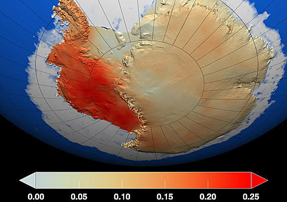
Map of warming across Antarctic that was recorded in Steigs study. Scale represents degrees celcius per decade.

This caused ripples throughout the climate denier community. Global warming skeptics have pointed to Antarctica in questioning the reliability of the models because of the mismatch between the data and the models. A quick web search reveals accusations of fraud and bitter name calling. A blog that is supported by many top climate scientists to try and explain and debunk mnay of the issues raised by climate deniers is Real Climate. Have a look at the debate to get a sense of the passion in this field....Real climate debate

Below is the video produced by Nature on Steigs paper which is in your resources.

Monday, November 29, 2010

Getting warmer....warmer...now you're hot


Curator Chad Broyles (IODP-USIO/TAMU; back to camera), Expedition Project Manager and Staff Scientist Jörg Geldmacher (IODP-USIO/TAMU), Co-Chief Scientist Takashi Sano (National Museum of Nature and Science, Japan), and Co-Chief Scientist Will Sager (TAMU) discuss a core recovered from Shatsky Rise. (Credit: John Beck, IODP/TAMU)

Will Sager is a professor at Texas Agricultural and Mechanical University (TAMU) in College Station. When I invited him to speak he was bobbing about in a small boat in the Indian Ocean doing seismic surveys - and didn't seem quite as enthused about the experience as he expresses on his web page.

'Dr. Sager’s research is broadly about Earth history, plate tectonics, and the evolution of ocean basins. He is a marine geophysicist who loves to explore the ocean and has been on 38 research cruises and was chief scientist on 17 of them. He has participated on seven Ocean Drilling Program cruises and was co-chief scientist for two. His expeditions have taken him and his students to each of the big three oceans.'

Sager will be discussing the results from a recent cruise to the Shatsky Rise in the northwest Pacific where they were examining hot spot volcanism. Hot spots are taught in entry level plate tectonics classes as an important piece of evidence to support the global theory of plate tectonics. In geology, a hot spot is a portion of the Earth's surface that is far from tectonic plate boundaries where volcanism occurs due to a rising mantle plume or some other cause.


Figure showing the three basic types of volcanism on the planet and the mantle behaviour beneath those volcanoes.

Plumes were once thought to have formed most seamount chains, but today it is thought that classic, deep-rooted mantle plumes are rare. The 145 million-year-old Shatsky Rise seamount chain has some characteristics that fit the plume-head hypothesis however other scientists suggest its formation is linked to spreading ridges (B in the figure above - creation of new ocean floor) and a triple junction. Located ~1500 kilometers (930 miles) east of Japan, Shatsky Rise measures roughly the size of California. This underwater mountain chain is one of the largest supervolcanoes in the world: the top of Shatsky Rise lies three and a half kilometers below the sea surface, while its base plunges to nearly six kilometers below the surface. Shatsky Rise is composed of layers of basalt, with individual lava flows (now hardened) that are up to 23 meters thick.


Map of the North Pacific showing the hotpot track of the Hawaiian and Emperor sea mount chains. To the west of the Emperor Chain is the Shatsky Rise (SR on the map). The map also shows trenches to the north and west of the chains.

According to Sager, Shatsky Rise is unique in that
'it is the only supervolcano to have formed during a time when Earth’s magnetic field reversed frequently.” This process creates “magnetic stripe” patterns in the seafloor. We can use these magnetic stripes to decipher the timing of the eruption and the spatial relationship of Shatsky Rise to the surrounding tectonic plates and triple junctions.'

On Friday Sager will discuss the expedition results, seamounts and plateaus of the Pacific, and his changing views on hotspots.

Tuesday, November 16, 2010

Sharpening the tools in the carbon dioxide garden shed


This weeks Smith Lecturer is Barbel Honisch, a tenure-track geochemist at Lamont-Doherty Earth Observatory (Columbia University). Lamont is center for research on Earth and ocean processes with a strong emphasis on climate. Like last weeks speaker Honisch is both German (which is irrelevant) and interested in reconstructing past ocean pH and atmospheric CO2 levels. Honisch was initially trained as a marine biologist, so she approaches ocean history questions with biological in mind. She is specifically interested in using boron isotopes as an indicator of past seawater pH. To check if calcium carbonate organisms are recording the pH of the seawater they float in correctly, Honisch has grown these organisms (foraminifera) in the lab.

Boron isotopes in marine carbonates have the potential to provide us with information about past ocean carbonate chemistry, as the boron isotopic composition of marine carbonates is primarily controlled by the pH of seawater. The boron isotope paleoacidity indicator is that the uncharged species B(OH)3 is enriched in 11B by 20% over the charged species B(OH)4-. As the fraction of boron changes with pH, so must the isotope.

11B(OH)3 + 10B(OH)4- double arrow 10B(OH)3 + 11B(OH)4-

Boron isotopes alone provide us with only one parameter (i.e. pH) of the marine carbonate system. For accurately translating boron isotope data into pH values and subsequently for calculating other parameters of the carbonate system such as aqueous PCO2, we need additional information on temperature, salinity and a second carbonate parameter such as carbonate ion concentration or alkalinity (the amount of carbonate ion).


Logic diagram shows how seawater pH (on the left) influences the ratio of stable isotopes of boron in corals that grew in that water (on the right). From Chacko (2009)
Application of the boron isotope pH proxy to the late Pleistocene ice ages has led to a convincing estimation of surface ocean pH that can be compared to atmospheric pCO2 as recorded in ice cores. Now Honisch is in the process of extending the pH and pCO2 reconstructions beyond the reach of ice records, into the Cenozoic era. The first application beyond the reach of ice core CO2 measurements focused on the mid-Pleistocene transition when the ice ages became significantly longer in length and duration. Her results suggest that although CO2 and climate were tightly coupled, the climate transition was not driven by an overall decrease in atmospheric CO2 that could have cooled the planet.

Video about growing 'pets' that will tell you about climate change through time.

Monday, November 8, 2010

'Look what you've done!! I'm melting, melting....'


Danni Schmidt is a Royal Society University Research Fellow at the University of Bristol is this weeks Smith lecturer. She writes
'I have always been deeply in love with the ocean (though I grew up in a rather land locked part of Germany) and hence studied Marine Geology at the University of Bremen and the Alfred Wegener Institute for Marine and Polar Research. During my time at AWI, I went to the Southern Ocean and knew that I want to continue studying the Ocean, its environments and how climate change is affecting life. During my PhD at ETH Zurich I studied the effect of biotic interaction and climate change on plankton evolution. Currently, my work is focussing on calcification and ocean acidification – past and future”. I am trying to inform policy decisons by contributing to the Marine Climate Change Impact Plan (UK) and by being a Lead author for the Working Group II of IPCC on the open ocean chapter. '


Schmidt will be talking about a hot new topic in Earth system science - ocean acidification. Another impact of raising atmospheric CO2 levels is the diffusion of atmospheric CO2 into water. About 1/3 of the CO2 we pump into the atmosphere dissolves in sea water (pCO2) where it dissociates into bicarbonate (HCO3) and carbonate (CO3) releasing H ions as it does so. Acidity or pH measures the number of H ions in water, as the number goes up, pH goes down (pH =-log10(H+) ). It is estimated that since the start of the industrial revolution (1750) ocean pH has dropped from 8.179 to 8.104.


Estimated change in annual mean sea surface pH between the pre-industrial period (1700s) and the present day (1990s). Δ pH here is in standard pH units.

The problem with this is that many marine organisms make their skeletons out of calcium carbonate (CaCO3). Different arrangements of CaCO3 molecules produce different minerals of calcium carbonate. For example aragonite is an arrangement that is physically strong and is favored by corals, but is chemically weak (dissolves easily), while calcite is chemically stronger and is favored by foraminifera and coccolithosphores. As pH drops these organisms will need to use more energy to build and prevent their shell from dissolving. The stress this causes can be seen in the misshapen shells/skeletons of these organisms.

Schmidt will be talking about other time periods in the past when CO2 levels were high. These intervals are perfect laboratories to examine the response of the ocean to higher pHs. Her research has shown that the change in ocean pH is happening faster than previous time intervals. Schmidt and her collaborators applied a model that compared current rates of ocean acidification with the greenhouse event at the Paleocene-Eocene boundary, about 55 million years ago when surface ocean temperatures rose by around 5-6°C over a few thousand years. During this event, no catastrophe is seen in surface ecosystems, such as plankton (the planktonic foraminifera and coccolithosphorids), yet bottom-dwelling organisms in the deep ocean experienced a major extinction. This is because the cold deep waters of the ocean can dissolve far more CO2 than the surface waters, making the deep ocean realm susceptible to rapid and extreme acidification. The occurrence of widespread extinction of these organisms during the Paleocene-Eocenegreenhouse warming and acidification event raises the possibility of a similar extinction in the future.

Monday, November 1, 2010

The Critical Zone - need I say more


This weeks Smith Lecturer is Suzanne Anderson from the University of Colorado, Boulder. Anderson's research uses field work to understand the mechanisms by which chemical and physical processes shape the Earth's surface and control chemical weathering and erosion. She will be focusing on the Critical Zone - a term that is coming into wide use to describe the layer of loose, heterogeneous material covering solid rock, and includes vegetation, the water table and water bodies. Within this zone a number of physical, chemical, and biological processes and reactions occur that impact mass and energy exchange necessary for biomass productivity, chemical recycling, and water storage. The concept of the Critical Zone unifies many complex biogeochemical and physical geologic processes in an attempt to create a numeric value from which predictions can be made. Why might this be important? You might want to make predictions based on the Critical Zone if you were interested in understanding how contaminants (heavy metals, radioactive material and other pollutents) might spread through the environment for example. This weeks reading is a review paper Anderson wrote for the magazine 'Elements'. This magazine is produced for a number of minerological and gechemical societies, with each issue exploring broad and current themes in the mineral sciences.

Monday, October 25, 2010

Tropical rainforests on the deep sea floor?


Professor Kai Hinrichs is coming from Germany to talk to us about archaea (single celled, microrganisms with no cell nucleus or organelles) on the bottom of the ocean. He describes himself as

'a biogeochemist studying the interactions between microbial life and the carbon cycle on a range of spatial, temporal and molecular scales. I am interested in which and how microbes shape element cycles and what the related environmental consequences are. In order identify and ideally quantify microbial processes, my research group studies the information encoded in distributions and isotopic compositions of organic biomarker molecules in geological and environmental samples, ranging in size from 1 to ~100 C-atoms. My group consists of closely collaborating biologists, chemists, geochemists, and marine geoscientists. In our research projects, we combine analyses of environmental samples with experimental, laboratory-based approaches. Our current research foci encompass the deep subsurface biosphere, methane biogeochemistry, life in extreme environments, development and application of new geochemical-analytical techniques, prokaryotic membrane lipid taxonomy, and the study of paleoenvironments associated with major perturbations of the C-cycle.'

The reading this week is an early nature paper Hinrich wrote discussing the decomposition of a methane hydrate (ice forming in sediment that contains large amounts of methane ), where the methane is being consumed by archaea. As no organism can consume methane without oxygen being present, scientists think that the consumption of methane must be done with a consortium of bacteria with some being sulfate (SO4) reducing (providing the oxygen) and some being a reverse type of methanogen (consuming methane rather than producing it). Hinrichs shows using very negative carbon isotopes that his archaea are feeding on methane and he suggests methane consuming archaea have evolved alongside methane producing archaea. Their presence is important if you want to estimate future or past methane concentrations in the atmosphere (faint sun paradox or at Permian-Triassic Boundary)- because when balancing carbon reservoirs consumption is just as important as production.

Tuesday, October 19, 2010

We're not in Kansas anymore....


This weeks lecturer will be discussing early Earth - going back in time to the point at which the first whiff of oxygen appeared.

The Hadean Era was the first in Earth history, extending from the first formation of continental crust, which began some time around 4.4 billion years becoming persistent soon after, to approximately 3.5 billion years. The earliest terrestrial environments were harsh: Levels of atmospheric oxygen around 1% were too low to sustain an ozone layer, without which there would have been little protection from solar radiation. High levels of atmospheric carbon dioxide and methane would have created a strong greenhouse effect, with global temperatures estimated to have been between 30 and 50°C. Oceans formed early, between 4.4 and 3.9 billion years, from condensation of atmospheric water vapor. Estimates suggest that the earliest oceans were hot (between 80 and 100°C) and acidic.

University of Colorado researcher Stephen Mojzsis explains what Earth might have looked like back then:

"Before 4 billion years ago, the Earth would not be recognizable for the pale blue world that we are familiar with today. Indeed, although we now understand that there were significant landmasses already present by that time, the denser carbon dioxide-rich atmosphere would have given the sky a reddish-tinge. The oceans, with a much higher concentration of iron than our contemporary oceans, would look a dark greenish-blue and these oceans would have bathed hundreds of small continents akin to New Zealand or the Japan arc,"

This weeks reading is a paper published by Mojzsis about evidence for life on earth at 3.4 billion years ago. Mojzsis measured carbon isotopes in inclusions within apatite grains. The isotopes (δ13C) were light – meaning they were enriched in 12C relative to 13C. Organisms turning CO2 into organic matter favor the 12C atoms over the 13C atoms because metabolic processes involving the lighter isotope occur faster. So inorganic carbon (C not fixed by organisms) has a δ13C of ~-10‰, carbonaceous fossils have a δ13C of ~-20 to -35‰ and photosynthesizers, ~-50 to -60‰.

Monday, October 11, 2010

The 'Canfield Ocean' Guy

You've made it when you have an ocean named after you or you have a wikipedia page (albeit a short one). The "Canfield Ocean", a sulfidic, partially oxic ocean existing for more than 40% of Earth history, between the Archean and Ediacaran periods, takes its name from his seminal paper (Nature, 1998). This finding has profound implications for biological evolution, and the history of atmospheric oxygen, carbonate sedimentology and climate. Canfield and his co-workers found convincing evidence that a prolonged, stable, oxygen-rich environment following the demise of the Canfield Ocean permitted the emergence of animals capable of movement some 550 million years ago. In Dons own words
"Fossil evidence suggests that animals probably evolved sometime around 600 million years ago, and large animals appear around 575 million years ago. Animals have an absolute requirement for oxygen for their respiration, so it has often been speculated that large macroscopic animals (those with the largest oxygen requirement) evolved when oxygen rose to permissible levels, which would be about 10% of those levels we have today. Our study supports this scenario by showing that the first occurrence of large respiring organisms, some of which are likely stem-group animals, emerged on the Avalon Peninsula in Newfoundland in concordance with oxygenation of this local environment."

On Friday Don will be talking about Oxygen Minimum Zones. The Oxygen minimum zone (OMZ), is the zone in which oxygen saturation in seawater in the ocean is at its lowest. This zone occurs at depths of about 200 to 1,000 metres, depending on location. Surface ocean waters generally have O2 concentrations in equilibrium with the atmosphere. Colder waters can hold more oxygen than warmer waters. As this water sinks from the surface into deeper waters it is exposed to a rain of organic matter from above. As aerobic bacteria feed on this organic matter they use oxygen as part of the bacterial metabolic process lowering its concentration within the surrounding water. Therefore, the concentration of oxygen in deep water is dependent on the amount of oxygen it had when it was at the surface minus depletion by the degradation of organic matter. The OMZ relates to new ways scientists are looking at the 'Great Oxygenation Event'.

The reading this week is another scientific paper which puts forward the idea the delivery of nutrients to the ocean following the last of the Snowball Earth Ice Ages (the Gaskiers glaciation) feed an algal (cyanobacterial) bloom that provided enough oxygen to fuel multicellular life - in other words animals. Don and his co-authors come up with this idea because the geochemistry of sediments before the Gaskiers glaciation is different from the geochemistry of the sediments afterwards.

Video primer about oxygen and photosynthesis

Tuesday, October 5, 2010

The Extinction happened on Tuesday at 9:15am

Sam Bowring is a professor at MIT who specializes in Uranium-lead zircon geochronology and has gotten really good at it. The precision that he is getting on his dates are amazing. Basically zircon is a mineral (ZrSiO4) that accepts element such as U which has a large ionic radius into its structure, but rejects Pb (lead). Zircon has an almost ubiquitous presence in the crust of Earth. It occurs in igneous rocks (as primary crystallization products), in metamorphic rocks and in sedimentary rocks (as detrital grains). U-Pb dating provides an age range of about 1 million years to over 4.5 billion years, and with routine precisions in the 0.1-1 percent range. The method relies on two separate decay chains, the uranium series from 238U to 206Pb, with a half-life of 4.47 billion years and the actinium series from 235U to 207Pb, with a half-life of 704 million years. Sam will be talking about two major extinctions that occurred on Earth.

Permo-Triassic Extinctions
A major extinction event occurred approximately 250 million years ago and marks the boundary between the Permian Period and the Triassic Period. At the end of the Permian more than 85% of all species in the oceans, approximately 70% of land vertebrates, and significant numbers of plants and insects vanished. The Permian extinction caused the most fundamental reorganization of ecosystems and animal diversity in the past 500 million years. The marine communities of today are largely a result of the recovery following this extinction. In addition, dinosaurs and mammals arose in the aftermath of the extinction.

A better understanding of how long the end-Permian extinction and its recovery took will allow for new insights and better understanding into the role of mass extinctions in evolution. Mass extinctions are marked in the fossil record by the abrupt disappearance of taxa, sometimes associated with a discrete "boundary bed"; in the case of the end Cretaceous extinction this bed is a layer rich in impact ejecta with distinctive chemical signatures. A critical question is how abrupt such extinctions really were. A satisfactory answer must involve statistical analysis of the stratigraphic and fossil record. Differences in sediment accumulation rate and the preservation potential of organisms can lead to an artificially abrupt and/or drawn out extinction signal, especially if the extinction is of short duration, say, less than 1 million years. Because sedimentation rates vary, stratigraphic thickness does not convert to time directly. Therefore, understanding an extinction requires constraining its tempo by combining high-precision geochronology with paleontological studies. Sam has found that the carbon isotope event associated with the major shift in carbon reservoirs as organisms disappeared from the planet was 165 thousand years long which indicates that there was a catastrophic addition of 12-carbon into the earths system. Furthermore he has found that most of the extinctions occurred in less than 1 milion years.

P-T Video featuring Sam Bowring


Monday, September 27, 2010

monkey, monkey, where for art thou monkey

Iyad Zalmout was born in Syria. He developed a love for geology growing up in the mountains collecting fossil gastropods and bivalves to show his friends - this later morphed into collecting lizards and snakes to scare his class mates. Iyad completed his PhD at the University of Michgan with Phil Gingrich on "Late Eocene sea cows (Mammalia, Sirenia) from Wadi al Hitan in the Fayum Basin, Egypt" and has stayed as a Post-doc in the Exhibit Museum.

A year ago Iyad was looking for whale fossils in a presumed to be section of marine sediments when he began to discover terrestrial mammal fossils. He was amazed to discover what is problably the last common ancestor of apes and monkeys before the two lineages separated. With a major discovery like this, press releases were made both by the publishing journal Nature and the University of Michigan. The reading this week will be the paper published in Nature.

Slide show of the primate fossils
Nature Video

Monday, September 20, 2010

Hydrothermal activity blasts out sediment


Ted Moore is an Emeritus Professor in the Department of Geological Sciences at the University of Michigan. This position is given to a professor who has retired but is highly regarded by the department. With this title Ted has some office and research space which allows him to continue research, which he has very actively. Since he retired he has sailed on research cruises, completed lecture tours and written papers. Ted was a pioneer in the field of paleoceanography and was integral to a massive community-based research initiative called CLIMAP, whose purpose was to map out the temperatures on the planet during the last ice age, 21 thousand years ago. Ted has a speciality in micropaleontology looking a a zooplankton group known as radiolaria. Radiolaria are a amoeboid protozoa that produce intricate skeletons made of silica.

Image of radiolaria from Nest Labs at the University of Dayton.

Ted will be talking about the sediments that are deposited in the equatorial region and their interaction with hydrothermal fluid. The classic hydrothermal vent in the ocean is associated with volcanism at mid ocean ridges (sea floor spreading centers at divergent boundaries). However a recent estimate (Bekins et al. 2007 - in resources) suggests that hydrothermal fluids exiting outcrops (cliffs) of basement (meaning the rock underlying sediment) sea floor (basalt generated at mid ocean ridges) may account for 75% of the hydrothermal outflow in the equatorial Pacific. These environments have become the focus of interest by scientist interested in microrganisms - these environments maybe similar to those found on other planets and the work these microrganisms do might be very important to the formation of mineral deposits.

Cartoons illustrating the development of pits over a bedrock outcrop. (a-c) show where flanking basins have approximately the same thickness of fill and (d-f) show where the basin fill is asymmetrical.

Ted came up with the model by which pits form in deep sea sediments allowing the discharge of waters circulating through the ocean crust. This water is able to remove heat from the cooling newly formed ocean plate explaining the low heat of the equatorial Pacific plates. The model suggests that the sediments overlaying the bedrock outcrop are dissolved by the water being discharged leaving behind sediment pits. These hydrothermal discharges may also be involved in the diagenetic alteration of siliceous sediments such as those which form from the remains of radiolaria. At high temperatures the silica remains of organisms convert to porcelanite and chert as the crystal structure of the opaline or biogenic silica changes.

Chert or jasper in the jasper conglomerate outside the CC Little building

Friday, September 10, 2010

Bedrock rivers and active deformation

Brian Yanites is a Post-doctoral Researcher in the Department of Geological Sciences at the University of Michigan. Brian did his PhD in Boulder at the University of Colorado with Greg Tucker.

Brian is interested in geomorphology - geologic research tries to understand the origin of the landforms (mountains, rivers etc) on Earth. On his web page he says he is trying to answer two fundamental questions: 1) How do local processes interact to form landforms and landscapes? and 2) How can we, as researchers, appropriately model and constrain these processes to explore the long-term evolution of the earth’s surface?

On Friday Brian will be talking about how to use river incision to understand deformation. Let's break that down. River incision refers to a river eroding downward through its riverbed which may be made of sediment or bedrock.The river begins at a higher elevation and incises or cuts or erodes downward through the bed it flows over. The river may leave its floodplain behind at a higher elevation of it may be lowered at the same time. Deformation refers to changes in the shape or volume of a rock body. Stress/pressure is often applied to rock bodies by plate tectonics for example. Rock bodies may bend in a ductile fashion (forming anticlines or synclines) or in a brittle fashion (faults that fracture rock bodies).

Rail lines outside Christchurch, New Zealand deformed in a ductile fashion in response of the earthquake of September 3rd 2010 (photo by Ian McGregor).

As the rock body under a river deforms, the river bed responds by becoming steeper (the elevation change down the river bed increases) and the width of the river bed becomes narrower (less distance between either side of the river bank). Both responses cause the river to become more erosive and the river will incise or cut down through its river bed faster. If the age of the beginning of the incision/cutting down is known, then the geomorphologist can calculate how quickly the river is eroding its bedrock.

Brian will be talking about rivers that drain off the Tibetan plateau. He has calculated how fast the rivers are incising the landscape by dating the time when incision began. Brian has used known earthquakes events as well as optically stimulated luminescence (OSL) dating techniques to calculate when the river sediments last saw sunlight to date the beginning of incision. Using his results Brian has helped us further understand the tectonics that are actively shaping our planet.

You can read more about these techniques at 'Rivers crossing growing folds' or in the Yanites folder in resources on Ctools.

Wednesday, September 8, 2010

Introductions: September 10 2010

New faculty, postdoctral researchers and graduate students will be introduced in this weeks Smith Lecture. There will be no lecture discussion as a result.